
Since a computer can only deal with numbers, we have to map numbers to other things that we understand, like text characters. Continuous runs of the same text characters (and thus the same numbers) can be easily compressed. However, there must be more we can do to more efficiently use space. In this post we explore one such approach to more efficiently use space: Huffman encoding.
The Challenge
When we consider a text. The mapping from text to numbers that can be stored and transmitted is fixed. For example: the number A is represented by the number 65, B by 66, etcetera. Each character is thus represented by one byte (each of which consists of eight bits). Let’s say that we have some text that look like this:
AAABBC
These six characters would take up 6 bytes (which is 6*8 = 48 bits). That seems quite a lot given that we only need to distinguish three things. Each byte can take 256 values, but we don’t need all of them. Also since A is much more frequent than C, maybe we can make each A take up less space than each C. So summarizing we can do two things:
- Encode so that we only have 3 possible values instead of 256.
- Use shorter sequences of bits for more frequently occurring characters, like A.
Intermezzo: Mapping Characters
Here is a quick refresher in case the numbers and characters confuse you:
Well, first we have upper and lowercase of course, which doubles this to 52. Still, shy of 255 though. The first forty or so ASCII values are actually used for non-printable characters. For example: things like the backspace, tab or enter. Otherwise we wouldn’t have line breaks for example. There are also other ‘control’ characters.
Moving on: value 40 represents a space, and from there on we get more into the printable characters. First symbols and numbers, then all uppercase characters (starting from 65) and lowercase (from 97). The ASCII standard defines only the first 128 possible values (first 7 bits): 0 – 127.
The interpretation of the other 128 values historically varied between languages. However, the inconvenience of that led eventually to Unicode standard and the UTF-8 encoding. Which can encode many symbols from many languages. It is backward compatible with the first 128 ASCII codes and uses the last bit to encode longer sequences of up to four bytes per character. In this post, we’ll continue assuming eight bits (one byte) per character, which is the standard when using English.
Concept: Using Fewer Bits
Back to the challenge and our AAABBC sequence. Instead of using 8 bits to encode a character, we simply can use fewer. One bit can be set to 0 or 1, so we could distinguish two values. That’s not enough, since we have three things to represent (A, B and C). So we need at least two bits for this example. With two bits we have four possibilities: 00, 01, 10, and 11. That’s a bit (pun intended) more than we need, but it can work and satisfies the first goal. We could say for example A = 00, B = 01 and C = 10. Then we can encode the sequence AAABBC as:
00 00 00 01 01 10
Now we have used only 12 bits instead of the original 48! That is a compression ratio of 48 / 12 = 4. Meaning the encoded data is four times smaller than the original (25%). That’s great, but: can we do better?
Concept: Encoding Shorter Sequences
We still use the same amount of space for A as we do for C. Everything is encoded using two bits. What if we don’t use the same number of bits for each character, but instead try to use fewer. Let’s get back to the example sequence AAABBC.
Since A is the most frequent character, ideally we’d assign it just one bit. Let’s do that. Let’s say A = 0. We can now encode the first three A’s like this:
0 0 0
We still have the B’s and a C to consider. So we know that we can’t use 0 any more, so both have to start with a 1. In our four possible options we had 10 and 11. So let’s use that: B = 10 and C = 11. We now get the sequence:
0 0 0 10 10 11
Which is 9 bits in length. This gives us an even better compression ratio of 48 / 9 = 5.33. There’s two things to notice here:
- We cannot use the sequence 01, because we assigned 0 to output A, and then stop. If you don’t understand why at this point: don’t worry it will become more apparent in the next section.
- We can no longer just read two bits at a time. A different approach is required: we need to decode the sequence of bits.
Concept: Decoding
Say that we have such a sequence of 0s and 1s. We also need to be able to decode it again to recover the original message. Think of it this way, processing the bits from left to right, we have these steps to go through:
- If we encounter a 0 it must be an A.
- If we encounter a 1 it could be either a B or a C. So we need to read the next bit.
- If the next bit is a 0 (so we’ve seen 10) we should output a B
- If the next bit is a 1 (so we’ve seen 11) we should output a C
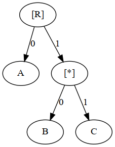
An easier way to see this is by using the tree below. Simply start at [R] and move through our sequence 0 0 0 10 11 (each time you go left or right depending on the position you are at). So we see the first three times we move left and output A. The fourth time we start again at [R] and then move right and then left and output B. Now there’s only 11 left, which I encourage you to trace from [R] yourself.
You can also see in the tree representation that the 1 acts as a prefix number for 10 and 11. Hence, 1 can not be used by itself. Hence the code 01 is invalid, as it would mean: output A, then move to [*] where there’s nothing to output. We need something else after 1 to determine if we should output B or C.
A More Complex Example
Let’s look at a more complex example with some real text. Let’s take the summary of Huffman’s paper that originally described his idea and encode it using his own method [1]:
“an optimum method of coding an ensemble of messages consisting of a finite number of members is developed. a minimum-redundancy code is one constructed in such a way that the average number of coding digits per message is minimized.”
– David A. Huffman
The table below shows the counts of the characters in the message. The top rows are the three characters that occur most throughout the text, these are two vowels and the ‘space’. The bottom three rows are the least common characters. The dash is used once for example to join the words minimum and redundancy.
| Character | Count |
| [SPC] | 38 |
| e | 25 |
| i | 18 |
| .. | .. |
| – | 1 |
| z | 1 |
| w | 1 |
Huffman Encoding the More Complex Example
The counts can be used to construct a tree, similar to what we did for the shorter example. This time we’ll follow the steps of Huffman’s algorithm, which works bottom up. First let’s define a ‘node’ as a combination of a character and a count, like a row in Table 1. Assume we have exactly that list of nodes. Now:
- Take two nodes with the lowest count and make them both children of a common parent node. Assign to this parent node the sum of the counts of the two child nodes. Since these two child nodes are now assigned, they will no longer be considered for this step.
- Repeat step 1 until there is only one node left. This is the root of the tree we can use for both encoding and decoding.
This example is too large to go through completely, but to illustrate let’s show two iterations of the first step.
- We first combine z (left) and w (right) under a common parent [*2] with count 2.
- Now the two lowest frequency items are this [*2] and the dash. Which we again combine with the dash (left) and the [*2] node, under a [*3] node.
Continuing to do this will give us a tree. The entire tree from the text is too large to include here. Instead the tree below is a partial one showing only the paths to the three most and three least frequent characters we identified in table one: [SPC], e, i, -, w and z.
The tree may look a bit more complex than it really is. There are 213 characters in total in the text. Starting from [R], the left part of the tree sums to 98, the right part to 133, and so on. The number thus refers to the count of characters represented by that part of the tree. At the very bottom of the left part, we find our [*2] and [*3] node we created in steps 1 and 2 above. Looking one level above this, we can see a [*6] node, from which we can infer that ‘p’ must occur 3 times (as 3 + 3 = 6). Indeed tracing back to [R] we see that the count roughly doubles each time we go up one level.
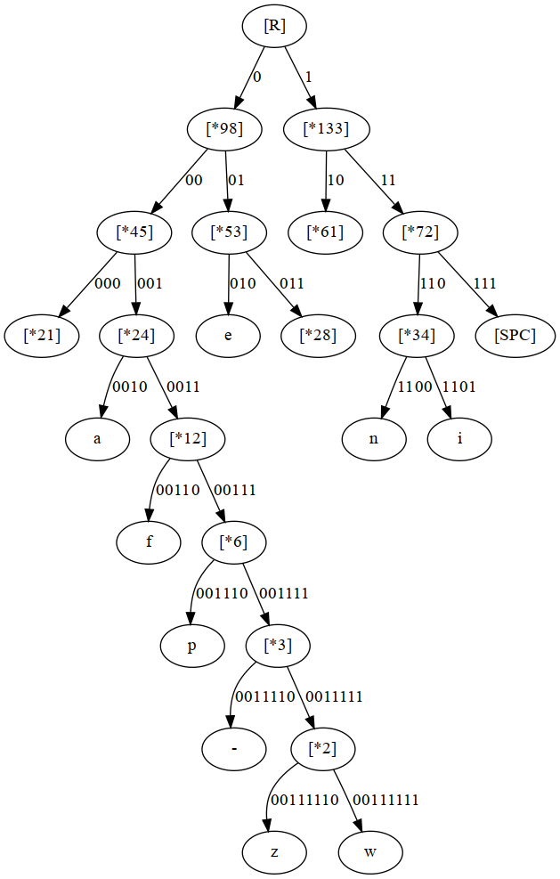
The tree also reveals the code themselves. We’d expect the characters with high counts to have a short code, and those with low counts to have long codes. From the tree, summarized in the table below, we can see this is indeed the case. The deeper we go in the tree, the longer the codes are. Hence, frequent characters live near the top of the tree and have a short path from [R].
| Character | Code |
| [SPC] | 111 |
| e | 010 |
| i | 1101 |
| .. | .. |
| – | 0011110 |
| z | 00111110 |
| w | 00111111 |
We can see that the tree has been built from the bottom up in this example, as we basically continue to combine the two nodes with the lowest count to form parts of the tree. This can also be done top down by starting by combining the nodes with the highest count. This is what we did in the first example, and it is called Shannon-Fano encoding [4]. However, it sometimes yields less optimal codes than Huffman encoding, and is thus rarely used in practice.
Huffman’s Background
David Huffman was told by his mother he lagged behind other children in learning to speak. He attributes his parent’s later divorce to incidents caused by his slow learning. However, this apparent slow start may have been a form of self-restraint or shyness.
Huffman later excelled academically and got his bachelor’s degree from Ohio state university when he was nineteen. He then spent two mandatory years in the navy on a destroyer. His captain resented him, and loaded him with duties to maximally leverage his engineering degree. After two years he went back to Ohio state to get his Master’s in Electrical Engineering and then applied to MIT in Boston, where he got in ‘by luck’.
He initially failed his doctoral examination, due to a lack of confidence and the culture shock of being in a different environment. Thinking of himself as a failure, he signed up, by accident, for a course in switching theory. A topic that would shape a significant part of the rest of his career.
The Epiphany of Huffman Encoding
The 25 year old Huffman did not want to take the standard final exam for the switching theory course. The alternative provided by his professor was to write a term paper about a classic coding problem: “Reduce the absolute minimum number of average yes/no questions necessary to identify one message out of a set of messages, when those messages may not appear with equal frequency”. His professor did not tell him and the other students that the optimal solution to this problem had evaded scientists up until then.
Finding the problem addictive, Huffman put in several months of effort. After that time he had no solution yet, and was about to throw his research notes in the trashcan. At that moment he realized he saw a pattern in what he had been doing, and wrote it down. It is what we now know as Huffman encoding, published as a paper in 1952. His professor was Robert Fano, who found that less optimal top-down approach to the same problem.
Huffman reflected that he might not even have tried solving the problem, had he been told that his professor, as well as Claude Shannon – the inventor of information theory, had been unsuccessful in trying to solve it. He would go on to make many other contributions, to both mathematics and computer science, before he passed away in 1999 at age 74.
Huffman Encoding: Algorithm Implementation
An entire implementation would be a bit too long for this post. The code excerpt below shows the most important parts, the steps to encode and decode, including the building and traversal of the tree structure. A complete implementation can be found here.
Note that this is a purely didactic implementation intended to aid understanding. In a real-world implementation, the bits would be set on actual bytes (not output to lists with 0’s and 1’s).
import heapq

class Node:
    def __init__(self, label, value, left=None, right=None):
        ....

class HuffmanEncoderDecoder:

    def _heap_to_encoding_tree(self, heap):
        # Builds a tree by occuring the two nodes with the
        # lowest count, until we have only one left, which is
        # the tree root.
        while len(heap) > 1:
            a = heapq.heappop(heap)
            b = heapq.heappop(heap)
            parent = Node(None, a.value + b.value, a, b)
            heapq.heappush(heap, parent)
        return heap[0]

    def encode(self, text):
        # Get (character, count) pairs and transform
        # to heap to easily get those with lowest count,
        # Then convert to an actual tree.
        counts = self._get_counts(text)
        heap = self._transform_to_heap(counts)
        root = self._heap_to_encoding_tree(heap)

        # Encode the text using the tree.
        bits = self._encode_bits(text, root)

        return bits, root

   def decode(self, bits, tree):
        # Iterate through the bits and step through the
        # tree, adding leaf labels to the output to
        # reconstruct the message.
        output = []
        current = tree
        for b in bits:
            if b == 0:
                current = current.left
            else:
                current = current.right
            if current.label:
                output.append(current.label)
                current = tree
        return "".join(output)
Conclusion
Huffman encoding is part of a family of entropy encoding approaches. Entropy may be an unfamiliar word, but it is basically the question posed by Huffman’s professor: “how many yes/no questions are needed to determine the content of a message?”. Huffman’s solution is optimal for this problem. That is: for when we are encoding a stream of symbols, like characters. More optimal approaches of entropy encoding exist that do not involve streams of symbols.
Huffman encoding has been with us for a long time, and is applied in for example fax machines, modems and televisions. It is also widely used as a part of more complex compression schemes. It can be found in file compression (ZIP, Brotli), compression of images (JPEG, PNG), audio (MP3), and transport mechanisms (HTTP/2).
Huffman’s discovery shows just what can happen if you sink your teeth into a problem and stay at it, not distracted by how others approached it so far. Huffman encoding provides an essential underpinning of present-day computing.
References
- Huffman, D. A. (1952). A Method for the Construction of Minimum-Redundancy Codes. Proceedings of the I.R.E., September 1952.
- Nelson, M & Gailly, J. (1996). The Data Compression Book.
- Stix, G. (1991). Encoding the Neatness of Ones and Zeroes. Scientific American, September 1991, pp. 54-58.
- Wikipedia (2020): Shannon-Fano Encoding, January 2021.
- Huffman, D. Biography.
- Huffman, K. Algorithm Description.